Inferencia Estadística

Pruebas de hipótesis

Author

Edimer David Jaramillo

Published

November 7, 2025

Bibliotecas

Code

library(tidyverse)
library(readxl)
library(infer)

theme_set(theme_bw())

Datos

Code

datos <- read_excel("datos-disexp/datos-encuestas-historia.xlsx")
datos

Escenarios de inferencia

Hipótesis estadística

Tipos de pruebas

Tipos de errores

Inferencia sobre una población

Inferencia sobre la media

Normalidad de la variable

Code

ggpubr::ggqqplot(datos$promedio_acad)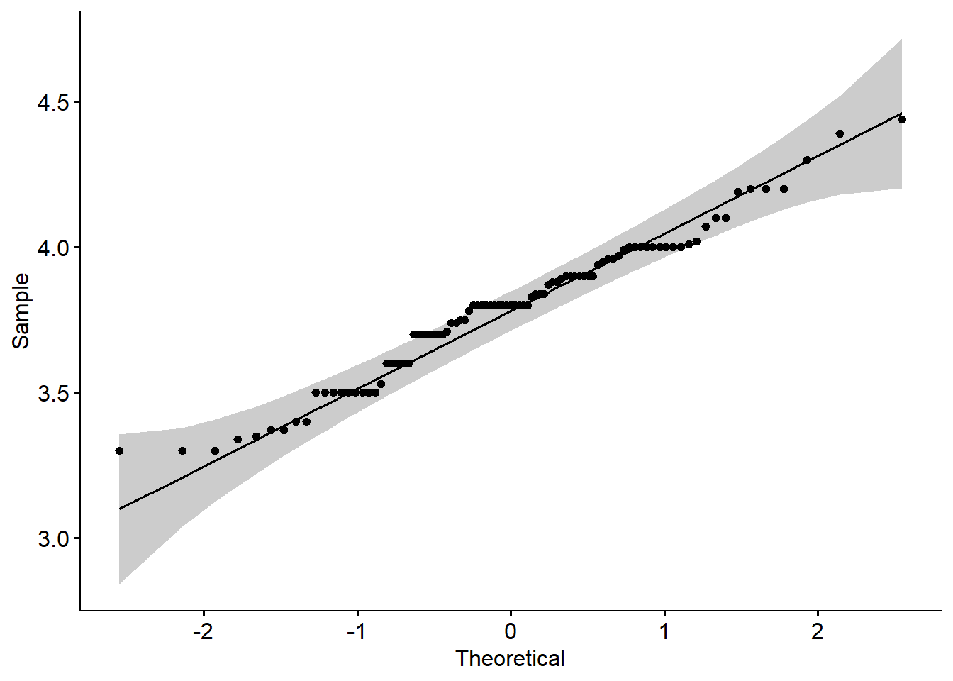

Juego de hipótesis

\[H_0: \mu = 3.5\]

\[H_1: \mu \neq 3.5\]

Nivel de significancia

Vamos a utilizar un nivel de significancia del 5% (\(\alpha = 0.05\))

Calcular el estadístico observado

En este caso calculamos el estadístico T:

\[T = \frac{\bar{X} - \mu}{S/\sqrt{n}}\]

Code

x_barra <- mean(datos$promedio_acad, na.rm = TRUE)
mu_referencia <- 3.5
desviacion_muestral <- sd(datos$promedio_acad, na.rm = TRUE)
raiz_n <- sqrt(nrow(datos))

\[T = \frac{3.794516 - 3.5}{0.247371/9.643651} = 11.48158\]

Code

(x_barra - mu_referencia) / (desviacion_muestral / raiz_n)

[1] 11.48158

Región de rechazo

Tabla t-student
Podemos obtener los límites critícos con R:

Code

qt(p = 0.025, df = 92, lower.tail = TRUE)

[1] -1.986086

Code

qt(p = 0.025, df = 92, lower.tail = FALSE)

[1] 1.986086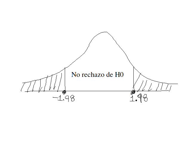

Conclusión: como el estadístico calculado (11.48158) está dentro de las regiones de rechazo, existe evidencia para rechazar la hipótesis nula, es decir, que se rechaza que el promedio del promedio_académico sea igual a 3.5. Esto se concluye con un nivel de significancia del 5%.

Intervalo de confianza para \(\mu\)

Límite inferior del intervalo de confianza:

\[\bar{X} - t_{\alpha/2, n-1} \times \frac{s}{\sqrt{n}}\]

Code

x_barra - (1.986086 * (desviacion_muestral / raiz_n))

[1] 3.743571

Límite superior del intervalo de confianza:

\[\bar{X} + t_{\alpha/2, n-1} \times \frac{s}{\sqrt{n}}\]

Code

x_barra + (1.986086 * (desviacion_muestral / raiz_n))

[1] 3.845462

Conclusión: como el valor de referencia (3.5) no está dentro del intervalo de confianza, existe evidencia para rechazar la hipótesis nula, es decir, que se rechaza que el promedio del promedio_académico sea igual a 3.5. Esto se concluye con un nivel de significancia del 5%. Como el intervalo de confianza está a la derecha del valor de referencia (3.5) podemos afirmar que la media del promedio académico de los estudiantes es mayor a 3.5

Valor p

Calcular el área que deja un valor de 11.48158 a la izquierda:

Code

pt(q = -11.48158, df = 92, lower.tail = TRUE)

[1] 9.287894e-20

Calcular el área que deja un valor de 11.48158 a la derecha:

Code

pt(q = 11.48158, df = 92, lower.tail = FALSE)

[1] 9.287894e-20

El valor p es la suma de las dor áreas anteriores:

Code

9.287894e-20 + 9.287894e-20

[1] 1.857579e-19

Conclusión: como el valor p (1.857579e-19) es menor que el nivel de significancia (0.05) existe evidencia para rechazar la hipótesis nula.

Solución con R

Utilizamos la función t.test() con los siguientes argumentos:
- x: la variable sobre la cual estamos haciendo inferencia. En este caso el promedio_académico
- alternative: tipo de hipótesis alternativa. En este es una prueba bilateral usamos “two.sided”
- conf.level: nivel de confianza (1 - nivel de significancia = 1 - 0.05 = 0.95)
- mu: valor promedio de referencia. En este caso es 3.5

Code

t.test(x = datos$promedio_acad,
       alternative = "two.sided",
       conf.level = 0.95,
       mu = 3.5)


    One Sample t-test

data:  datos$promedio_acad
t = 11.482, df = 92, p-value < 2.2e-16
alternative hypothesis: true mean is not equal to 3.5
95 percent confidence interval:
 3.743571 3.845462
sample estimates:
mean of x 
 3.794516

Presentando resultados de la prueba anterior, de forma ordenada (tidy):

Code

prueba_t1 <- t.test(
  x = datos$promedio_acad,
  alternative = "two.sided",
  conf.level = 0.95,
  mu = 3.5
)

library(broom)
prueba_t1 |> tidy()

Alternativa no parámetrica 1: Test de Wilcoxon

Test de Wilcoxon

Code

wilcox.test(
  x = datos$promedio_acad,
  alternative = "two.sided",
  conf.int = TRUE,
  conf.level = 0.95,
  mu = 3.5
)


    Wilcoxon signed rank test with continuity correction

data:  datos$promedio_acad
V = 3465.5, p-value = 6.357e-14
alternative hypothesis: true location is not equal to 3.5
95 percent confidence interval:
 3.794980 3.884976
sample estimates:
(pseudo)median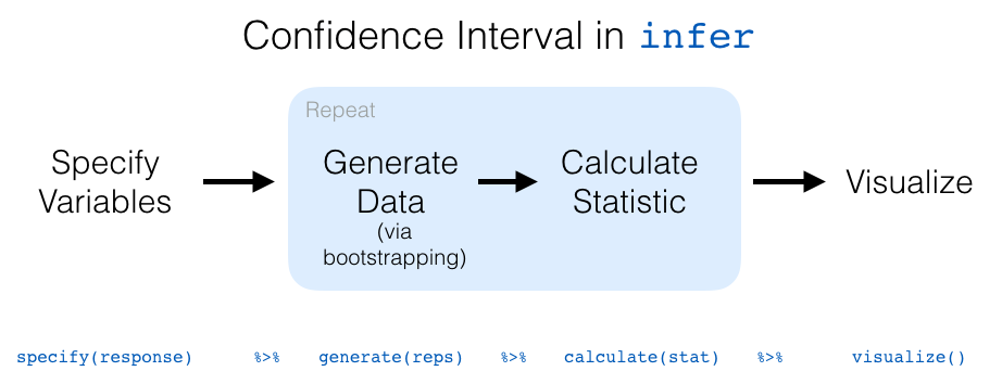 
       3.84006

Alternativa no parámetrica 2: Boootstrapping

Code

set.seed(2025)
bootstrap_promedio_udea <- 
  datos |> 
  specify(response = promedio_acad) |> 
  generate(reps = 1000, type = "bootstrap") |> 
  calculate(stat = "mean")

bootstrap_promedio_udea

Graficamos la distribución bootstrap:

Code

bootstrap_promedio_udea |> 
  visualize()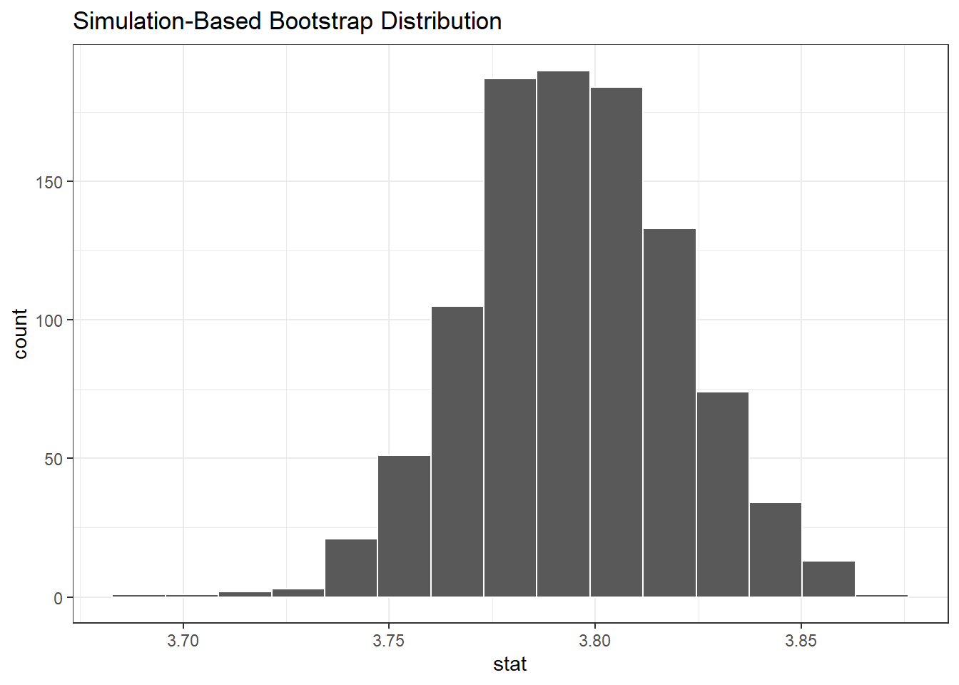

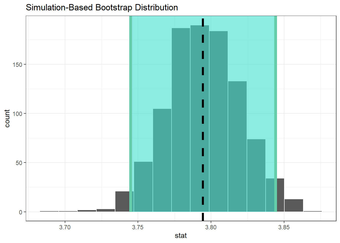
Intervalos de confianza

Método de percentiles

Intervalo de confianza con percentiles (95%):

Code

ic_promedio_percentil <-
  bootstrap_promedio_udea |> 
  get_confidence_interval(level = 0.95, type = "percentile")
ic_promedio_percentil

Graficamos el intervalo de confianza obtenido con el método de percentiles:

Code

bootstrap_promedio_udea |> 
  visualize() +
  shade_confidence_interval(endpoints = ic_promedio_percentil) +
  geom_vline(
    xintercept = x_barra,
    color = "red",
    lty = 2,
    size = 1.5
  ) +
  geom_vline(
    xintercept = mean(datos$promedio_acad),
    color = "black",
    lty = 2,
    size = 1.5
  )

Método de error estándar

Intervalo de confianza con método del error estándar:

Code

ic_promedio_error_est <-
  bootstrap_promedio_udea |> 
  get_confidence_interval(type = "se", point_estimate = x_barra)
ic_promedio_error_est

Graficamos el intervalo de confianza obtenido con el método de percentiles:

Code

bootstrap_promedio_udea |> 
  visualize() +
  shade_confidence_interval(endpoints = ic_promedio_error_est) +
  geom_vline(
    xintercept = x_barra,
    color = "red",
    lty = 2,
    size = 1.5
  ) +
  geom_vline(
    xintercept = mean(datos$promedio_acad),
    color = "black",
    lty = 2,
    size = 1.5
  )

Inferencia sobre 2 poblaciones

Inferencia sobre \(\sigma^2\)

Datos

Code

datos_cebada <- read_excel("datos-disexp/datos_cebada.xlsx") |> 
  mutate(year = as.factor(year))
datos_cebada

Hipótesis

\[H_0: \sigma^2_{1931} / \sigma^2_{1932} = 1\]

\[H_1: \sigma^2_{1931} / \sigma^2_{1932} \neq 1\]

Nivel de significancia

En este caso vamos a usar un nivel de significancia del 5%.

Analizando la normalidad

Gráfico:

Code

library(ggpubr)
ggqqplot(data = datos_cebada$yield)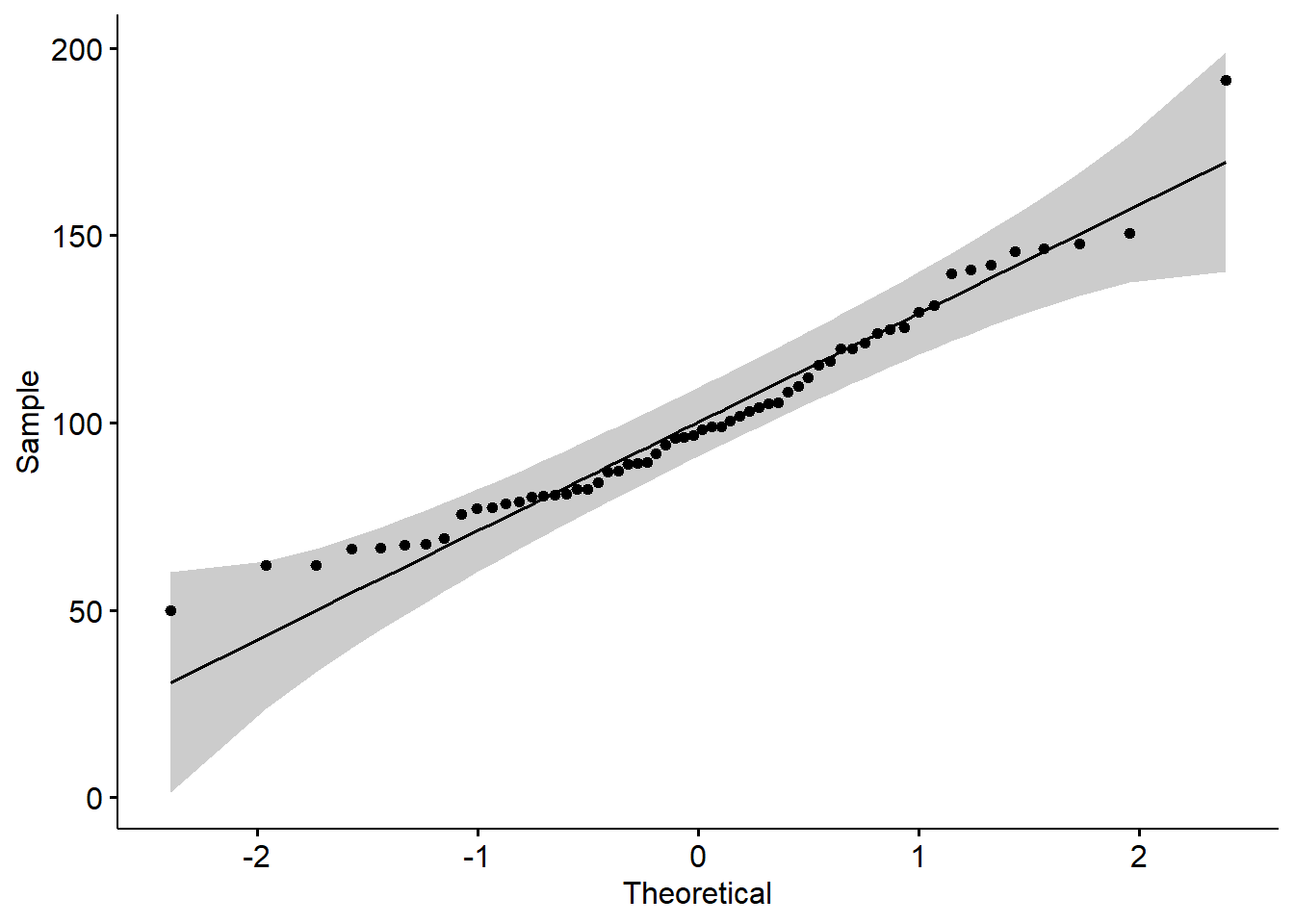

Prueba de shapiro wilk:

Code

shapiro.test(x = datos_cebada$yield)


    Shapiro-Wilk normality test

data:  datos_cebada$yield
W = 0.96055, p-value = 0.05005

Solución con R

Vamos a usar la función var.test() con los siguientes argumentos:
- formula: y ~ x. En este caso “y” es la variable produccion y el “x” es el año.
- ratio: es el resultado del cociente de las dos varianzas. En este caso asumimos en la hipótesis nula el valor de “1”.
- alternative: tipo de prueba. En este es bilateral (“two.sided”)
- conf.level: nivel de confianza. En este caso es 0.95 (1 - 0.5)

Code

var.test(datos_cebada$yield ~ datos_cebada$year,
         ratio = 1,
         alternative = "two.sided",
         conf.level = 0.95)


    F test to compare two variances

data:  datos_cebada$yield by datos_cebada$year
F = 1.3952, num df = 29, denom df = 29, p-value = 0.375
alternative hypothesis: true ratio of variances is not equal to 1
95 percent confidence interval:
 0.6640874 2.9314037
sample estimates:
ratio of variances 
          1.395245

Conclusión:
- Como el valor p (0.375) es mayor que el nivel de significancia (0.05), no existe evidencia para rechazar la hipótesis, es decir, que la varianza para la producción del año 1931 es igual a la varianza para la producción del año 1932.
- Como el intervalo de confianza (LI: 0.6640874, LS: 2.9314037) contiene el valor de referencia (“1”), no existe evidencia para rechazar la hipótesis.

Prueba de Bartlett

Esta prueba es recomendada para comparar varianzas cuando la normalidad se cumple.

Code

bartlett.test(datos_cebada$yield ~ datos_cebada$year)


    Bartlett test of homogeneity of variances

data:  datos_cebada$yield by datos_cebada$year
Bartlett's K-squared = 0.78702, df = 1, p-value = 0.375

Prueba de Levene

Esta prueba es recomendada para comparar varianzas cuando la normalidad no se cumple:

Code

library(car)
leveneTest(datos_cebada$yield ~ datos_cebada$year)

Inferencia sobre \(\mu_1 - \mu_2\)

Datos

Code

datos_trigo <- read_excel("datos-disexp/datos_trigo.xlsx")
datos_trigo

Hipótesis

\[H_0: \mu_{bajo} = \mu_{alto}\]

\[H1: \mu_{bajo} \neq \mu_{alto}\]

El juego de hipótesis anterior es equivalente al siguiente:

\[H_0: \mu_{bajo} - \mu_{alto} = 0\]

\[H1: \mu_{bajo} - \mu_{alto} \neq 0\]

Nivel de significancia

El nivel de significancia será del 5%.

Normalidad

Para la prueba t-student sobre dos poblaciones (medias) se debe garantizar que la variable (en cada grupo) se distribuye de forma normal.

Code

nitro_bajo <- datos_trigo |> filter(nitro == "L")
nitro_alto <- datos_trigo |> filter(nitro == "H")

ggqqplot(nitro_bajo$yield)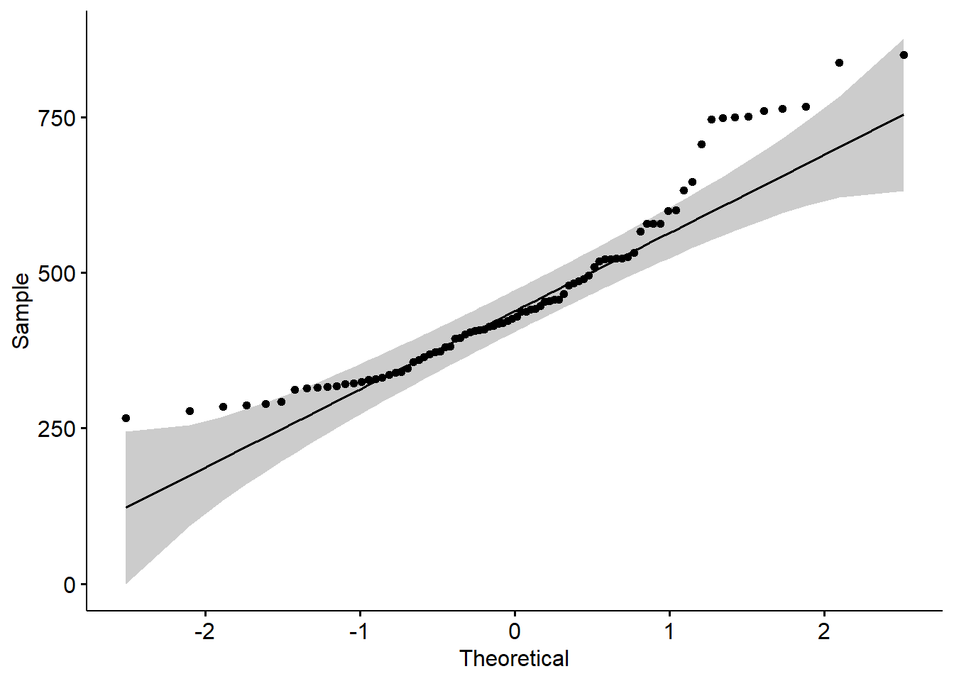

Code

ggqqplot(nitro_alto$yield)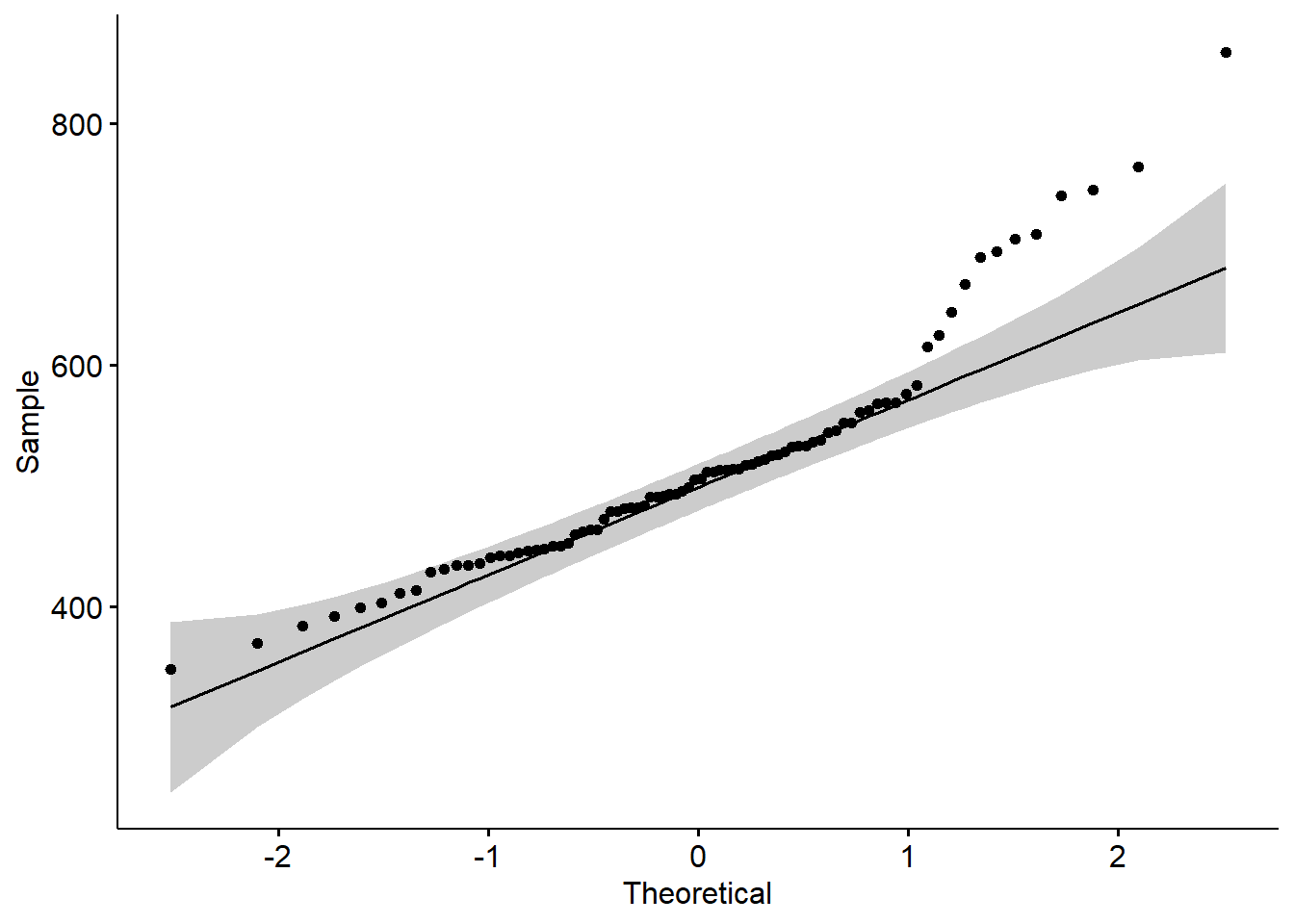

Pruebas de shapiro wilk:

Code

shapiro.test(nitro_alto$yield)


    Shapiro-Wilk normality test

data:  nitro_alto$yield
W = 0.90953, p-value = 2.064e-05

Code

shapiro.test(nitro_bajo$yield)


    Shapiro-Wilk normality test

data:  nitro_bajo$yield
W = 0.9039, p-value = 1.153e-05

Igualdad de varianzas

Como el valor p ( 0.001958 ) es menor que el nivel de significancia, existe evidencia para manifestar que las varianzas son diferentes para el grupo de nitrógeno alto y bajo.

Code

leveneTest(datos_trigo$yield ~ datos_trigo$nitro)

Solución con R

Usamos la función t.test() con los siguientes argumentos:
- formula: y ~ x. En este caso “y” es la producción y “x” es el nivel de fertilización con nitrógeno (bajo, alto)
- alternative: tipo de hipótesis alternativa. En este caso es bilateral.
- conf.level: nivel de confianza. En este caso es del 95%
- var.equal: toma valores TRUE o FALSE para cuando las varianzas son iguales o diferentes, respectivamente.
Nota: los supuestos matemáticos necesarios no se cumplen, por tal motivo se debe optar por algún método no paramétrico.

Code

t.test(datos_trigo$yield ~ datos_trigo$nitro,
       alternative = "two.sided",
       conf.level = 0.95,
       var.equal = FALSE)


    Welch Two Sample t-test

data:  datos_trigo$yield by datos_trigo$nitro
t = 2.9051, df = 143.36, p-value = 0.004254
alternative hypothesis: true difference in means between group H and group L is not equal to 0
95 percent confidence interval:
 17.44086 91.70200
sample estimates:
mean in group H mean in group L 
       517.4762        462.9048

Conclusión:
- Como el valor p (0.004254) es menor que el nivel de significancia (0.05), existe evidencia para rechazar la hipótesis nula, es decir, que el promedio de producción de bajo nitrógeno es diferente al promedio de producción de alto nitrógeno.
- Como el intervalo de confianza no contiene al cero, entonces existe evidencia para rechazar la hipótesis nula. Además, como el intervalo de confianza está a la derecha del cero, quiere decir que en promedio el grupo de alta dosificación estará por encima del promedio de baja dosificación en nitrógeno.

Inferencia sobre p1-p2

Hipótesis

\[H_0: p1 = p2\] \[H_1: p1 \neq p2\]

O de forma equivalente:

\[H_0: p1 - p2 = 0\]

\[H_1: p1 - p2 \neq 0\]

Nivel de significancia

En este caso usaremos un nivel de significancia del 5% (0.05)

Calculando proporciones

En este caso queremos comaparar la proporción de estudiantes que trabajan vs los que no trabajan.

Code

table(datos$trabaja)


No Sí 
71 22

Solución con R

Usamos la función prop.test() con los siguientes argumentos:
- x: el número de éxitos para el evento de interés. En este caso son estudiantes que trabajan (n = 21) y no trabajan (n = 71)
- n: total de ensayos (observaciones). En este caso equivale a 93.
- alternative: tipo de hipótesis alternativa. En este caso es “two.sided”
- conf.level: nivel de confianza. En este caso es 1 - 0.05 = 0.95

Code

prop.test(x = c(21, 71),
          n = c(93, 93),
          alternative = "two.sided",
          conf.level = 0.95)


    2-sample test for equality of proportions with continuity correction

data:  c(21, 71) out of c(93, 93)
X-squared = 51.64, df = 1, p-value = 6.666e-13
alternative hypothesis: two.sided
95 percent confidence interval:
 -0.6695517 -0.4057172
sample estimates:
   prop 1    prop 2 
0.2258065 0.7634409

Conclusión:
- Como el valor p (6.666e-13) es menor que el nivel de significancia (0.05), existe evidencia para rechazar la hipótesis nula, es decir, que la proporción de estudiantes que trabajan y no trabajan no es la misma.
- Como el intervalo de confianza para la diferencia de proporciones ([LI: -0.6695517 , LS: -0.4057172]) no contiene al cero, entonces existe evidencia para rechazar la hipótesis nula.

T-student medias pareadas

Datos

Code

calificaciones <- read_excel("datos-disexp/datos_parciales.xlsx")
calificaciones

Juego de hipótesis

\[H_0: \mu_{post} - \mu_{pre} = 0\]

\[H_1: \mu_{post} - \mu_{pre} \neq 0\]

Nivel de significancia

En este caso vamos a usar un nivel de significancia del 5% (0.05)

Diferencia de medias

Code

diferencia <- calificaciones$Post - calificaciones$Pre
diferencia

 [1]  4  4  1  2 -3  5  3  2 -4  2  1 -1  2  7  0  4  6  3  4 -1

Normalidad

Gráfico:

Code

ggqqplot(data = diferencia)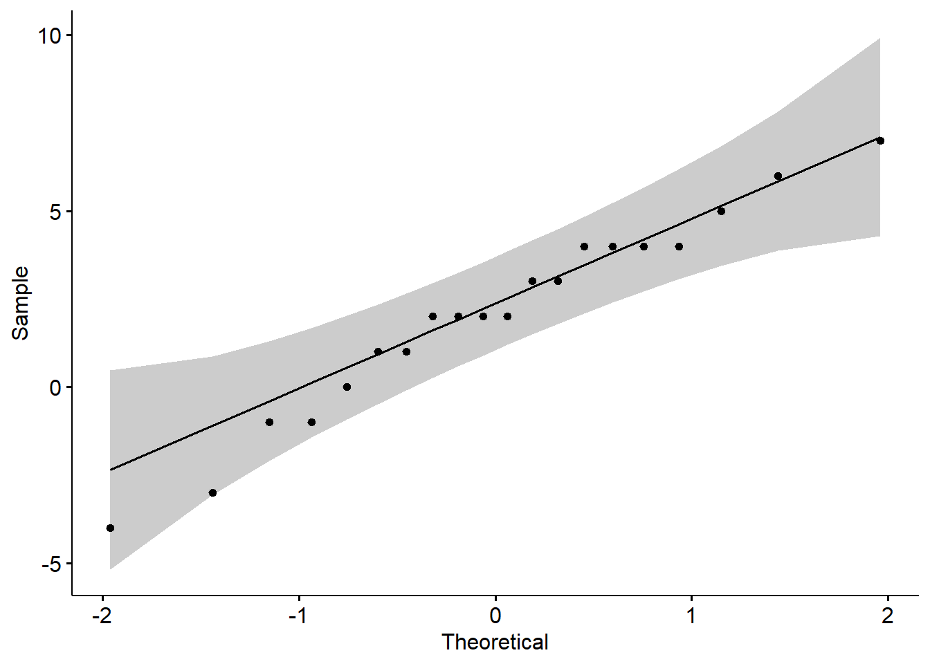

Shapiro Wilk: la normalidad se cumple (0.725)

Code

shapiro.test(x = diferencia)


    Shapiro-Wilk normality test

data:  diferencia
W = 0.9686, p-value = 0.725

Igualdad de varianzas

Existe igualdad de varianzas (0.2795)

Code

var.test(x = calificaciones$Pre,
         y = calificaciones$Post,
         ratio = 1,
         alternative = "two.sided",
         conf.level = 0.95)


    F test to compare two variances

data:  calificaciones$Pre and calificaciones$Post
F = 0.60329, num df = 19, denom df = 19, p-value = 0.2795
alternative hypothesis: true ratio of variances is not equal to 1
95 percent confidence interval:
 0.238790 1.524186
sample estimates:
ratio of variances 
         0.6032913

Prueba t-student

Code

t.test(x = calificaciones$Pre,
       y = calificaciones$Post,
       alternative = "two.sided",
       conf.level = 0.95,
       paired = TRUE,
       var.equal = TRUE)


    Paired t-test

data:  calificaciones$Pre and calificaciones$Post
t = -3.2313, df = 19, p-value = 0.004395
alternative hypothesis: true mean difference is not equal to 0
95 percent confidence interval:
 -3.3778749 -0.7221251
sample estimates:
mean difference 
          -2.05

Conclusión:
- Como el valor p (0.004395) es menor que el nivel de significancia, existe evidencia para rechazar la hipótesis nula, es decir, que el promedio del “post” es diferente al promedio para el “pre”.
- Como el intervalo de confianza está a la izquierda del cero ([-3.3778749, -0.7221251]), existe evidencia para rechazar la hipótesis nula. Además, el promedio del “pre” podría estar desde 0.72 hasta 3.37 puntos por debajo del “post”.

Referencia

Libro: Statistical Inference via Data Science: A ModernDive into R and the Tidyverse